テクノロジー業界には、AI (人工知能)、ML (機械学習)、DNN (ディープニューラルネットワーク)、CV (コンピュータービジョン)、CNN (畳み込みニューラルネットワーク)、RNN (リカレントニューラルネットワーク)などが氾濫しています。機械の知覚には、機械が視覚、聴覚、触覚、嗅覚、味覚の5つの感覚からのインプットを理解する能力が含まれていますが、機械の視覚においては、コンピュータビジョンとSLAMについて耳にされたことがあるかしれません。
SLAM、Computer Visionについて、概説します。(以下、英文のみ)
The technology industry is inundated with references to AI (artificial intelligence), ML (machine learning), DNN’s (deep neural networks), CV (computer vision), CNN’s (convolutional neural networks), RNN’s (recurrent neural networks), etc..
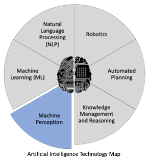
What these acronyms represent are some of the components that make up the field of Artificial Intelligence. Imagine an artificial being, and what it needs to successfully interact with the world around it - the ability to sense and perceive its environment (machine perception), the ability to understand speech (natural language processing), the ability to remember information, learn new things, and make inferences (machine learning, knowledge management and reasoning), the ability to plan and execute actions (automated planning), and the ability to interact with its environment (robotics).
Machine perception encompasses the capabilities enabling machines to understand the input from the 5 senses - visual, auditory, tactile, olfactory, and gustatory. (Yes, they do have machines that analyze smell and taste).
Computer Vision and SLAM
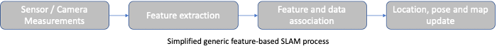
Buried among these acronyms, you may have come across references to computer vision and SLAM. Let’s dive into the arena of computer vision and where SLAM fits in. There are a number of different flavors of SLAM, such as topological, semantic and various hybrid approaches, but we’ll start with an illustration of metric SLAM.
As the name suggests (intuitively or not), Simultaneous Localization and Mapping is the capability for a machine agent to sense and create (and constantly update) a representation of its surrounding environment (this is the mapping part), and understand its position and orientation within that environment (this is the localization part). Most humans do this well enough without much effort, but trying to get a computer to do this is another matter.
There are many types of sensors that can detect the surrounding environment, including camera(s), Lidar, radar, and sonar. As the machine agent with the sensors (such as the ones listed prior) moves through space, a snapshot of the environment is created, while the relative position of the machine agent within that space is tracked. Thus, a picture is formed by features represented as points in space including the relative distance from the observer and with each other.
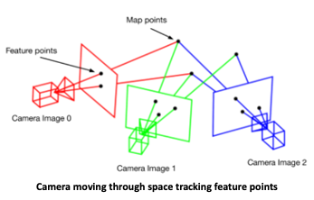
Over time, this collection of feature points and their registered position in space grow together to form a point cloud, a 3-dimensional representation of the environment. This is the “mapping” part in SLAM.
As the map is being created, the machine agent tracks its relative position and orientation within that point cloud, enabling the “localization” part in SLAM. Once a map is available, then any arbitrary machine agent using the map would be able to “relocalize” within that space - ie. determine its location on the map from what it perceives around it.
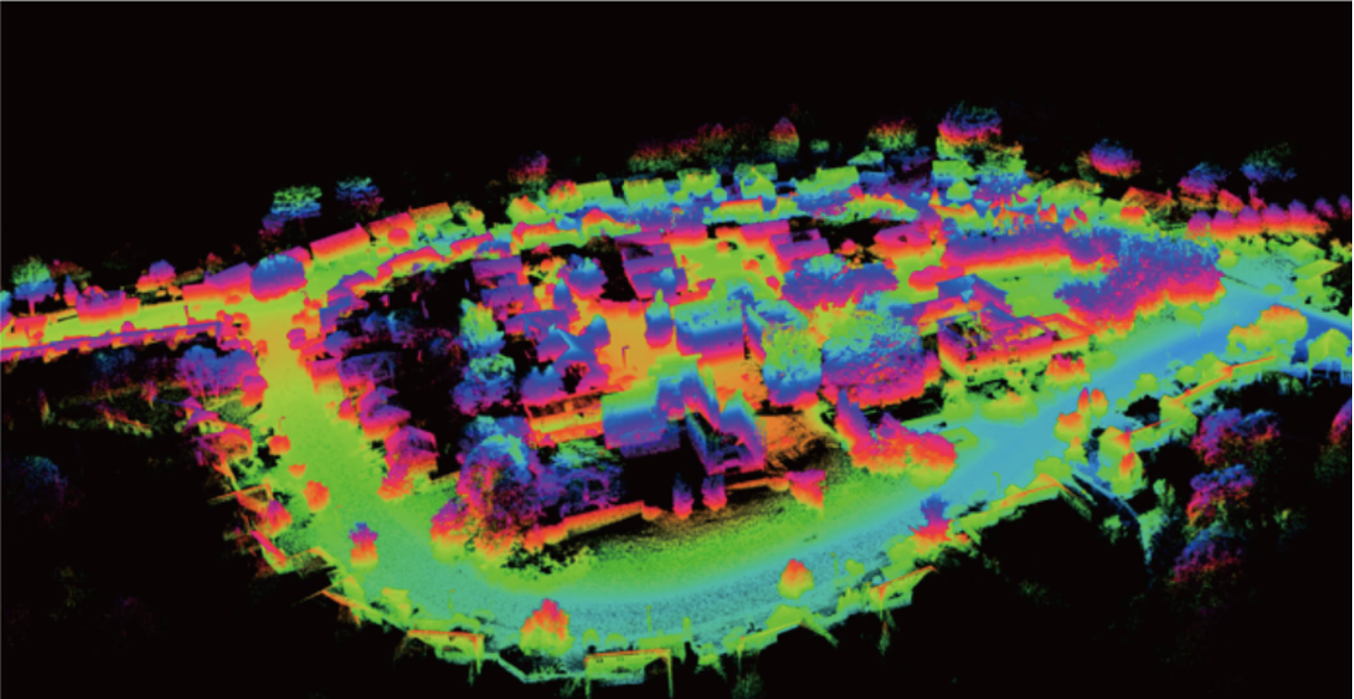
Point cloud model created using Lidar scans
Sounds simple enough
That doesn’t sound too hard, but let’s think about this from a processing perspective.
Let’s assume that we have a stereo camera system performing feature-based visual SLAM.
Now imagine a machine agent needing to keep track of hundreds or thousands of points, each with a level of error and drift that needs to be tracked and corrected, and the cameras continue to deliver 30 (or more) frames per second. With each frame, the agent estimates the depth or distance based on the disparity of images between your stereo camera images, looks for features within that image, matches it to previously tracked features, checks to see if the map can be looped/closed-ended, adds new features that are captured, and localizes the agent’s new position with regards to all the track features.
The figure below shows SLAM in action with the feature points highlighted in the central image as the video is captured, and the view of the map being constructed with those feature points in the top left corner along with the camera trajectory.
As you can imagine, this quickly becomes an optimization and approximation exercise for SLAM to run in real-time, or near real-time. Many of the initial applications of SLAM revolved around autonomous vehicles and autonomous robots, where the ability to navigate in an unfamiliar environment, while avoiding obstacles and collisions, in real-time was a critical requirement. As the series continues, I’ll explore various aspects of SLAM, such as Kalman filters, loop closure, bundle adjustment, etc., and delve into what Kudan does with our approach to SLAM. We will also dive into use cases and applications of SLAM and its challenges.
For further reading:
These are some of the early seminal works that defined SLAM in the 1980’s and 90’s.
Smith, R.C.; Cheeseman, P. (1986). "On the Representation and Estimation of Spatial Uncertainty" (PDF).
Smith, R.C.; Self, M.; Cheeseman, P. (1986). "Estimating Uncertain Spatial Relationships in Robotics" (PDF).
Leonard, J.J.; Durrant-whyte, H.F. (1991). "Simultaneous map building and localization for an autonomous mobile robot" (PDF).