本記事では、過去10年間のDirect Visual SLAMの進化と、そこから生まれたいくつかの興味深い傾向を具体的に見ていきます。
(以下、英文のみ)
In my last article, we looked at feature-based visual SLAM (or indirect visual SLAM), which utilizes a set of keyframes and feature points to construct the world around the sensor(s). This approach initially enabled visual SLAM to run in real-time on consumer-grade computers and mobile devices, but with increasing CPU processing and camera performance with lower noise, the desire for a denser point cloud representation of the world started to become tangible through Direct Photogrammetric SLAM (or Direct SLAM). A denser point cloud would enable a higher-accuracy 3D reconstruction of the world, more robust tracking especially in featureless environments, and changing scenery (from weather and lighting). In this article, we will specifically take a look at the evolution of direct SLAM methods over the last decade, and some interesting trends that have come out of that.
Direct SLAM started with the idea of using all the pixels from camera frame to camera frame to resolve the world around the sensor(s), relying on principles from photogrammetry. Instead of extracting feature points from the image and keeping track of those feature points in 3D space, direct methods look at some constrained aspects of a pixel (color, brightness, intensity gradient), and track the movement of those pixels from frame to frame. This approach changes the problem being solved from one of minimizing geometric reprojection errors, as in the case of indirect SLAM, to minimizing photometric errors.
The direct visual SLAM solutions we will review are from a monocular (single camera) perspective. Having a stereo camera system will simplify some of the calculations needed to derive depth while providing an accurate scale to the map without extensive calibration.
In the interest of brevity, I’ve linked to some explanations of fundamental concepts that come into play for visual SLAM:
While these ideas help in the deeper understanding of some of the mechanics, we’ll save them for another day.
Dense tracking and mapping (DTAM, 2011)
The DTAM approach was one of the first real-time direct visual SLAM implementations, but it relied heavily on the GPU to make this happen. Grossly simplified, DTAM starts by taking multiple stereo baselines for every pixel until the first keyframe is acquired and an initial depth map with stereo measurements is created. Using this initial map, the camera motion between frames is tracked by comparing the image against the model view generated from the map. With each successive image frame, depth information is estimated for each pixel and optimized by minimizing the total depth energy.
The result is a model with depth information for every pixel, as well as an estimate of camera pose. Since it is tracking every pixel, DTAM produces a much denser depth map, appears to be much more robust in featureless environments, and is better suited for dealing with varying focus and motion blur.
The following clips compare DTAM against Parallel Tracking and Mapping: PTAM, a classic feature-based visual SLAM method.
![]()
With rapid motion, you can see tracking deteriorate as the virtual object placed in the scene jumps around as the tracked feature points try to keep up with the shifting scene (right pane). DTAM on the other hand is fairly stable throughout the sequence since it is tracking the entire scene and not just the detected feature points.
Since indirect SLAM relies on detecting sharp features, as the scene’s focus changes, the tracked features disappear and tracking fails. This can occur in systems that have cameras that have variable/auto focus, and when the images blur due to motion.
In this instance, you can see the benefits of having a denser map, where an accurate 3D reconstruction of the scene becomes possible.
Source video: https://www.youtube.com/watch?v=Df9WhgibCQA
Visual odometry and SLAM
We will start seeing more references to visual odometry (VO) as we move forward, and I want to keep everyone on the same page in terms of terminology. As described in previous articles, visual SLAM is the process of localizing (understanding the current location and pose), and mapping the environment at the same time, using visual sensors. An important technique introduced by indirect visual SLAM (more specifically by Parallel Tracking and Mapping - PTAM), was parallelizing the tracking, mapping, and optimization tasks on to separate threads, where one thread is tracking, while the others build and optimize the map. For the purposes of this discussion, VO can be considered as focusing on the localization part of SLAM. The VO process will provide inputs that the machine uses to build a map. However, it will need additional functions for map consistency and optimization.
Large Scale Direct SLAM (LSD-SLAM, 2014)
Building on earlier work on the utilization of semi-dense depth maps for visual odometry, Jakob Engel (et al.), proposed the idea of Large Scale Direct SLAM. Instead of using all available pixels, LSD-SLAM looks at high-gradient regions of the scene (particularly edges) and analyzes the pixels within those regions. The idea being that there was very little to track between frames in low gradient or uniform pixel areas to estimate depth. For single cameras, the algorithm uses pixels from keyframes as the baseline for stereo depth calculations.
The following image highlights the regions that have high intensity gradients, which show up as lines or edges, unlike indirect SLAM which typically detects corners and blobs as features.
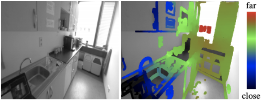 Image from Engel’s 2013 paper on “Semi-dense visual odometry for monocular camera
To complement the visual odometry into a SLAM solution, a pose-graph and its optimization was introduced, as well as loop closure to ensure map consistency with scale. In the following clip, you can see a semi-dense map being created, and loop closure in action with LSD-SLAM. You can see the map snap together as it connects the ends together when the camera returns to a location it previously mapped.
 Source video: https://www.youtube.com/watch?v=GnuQzP3gty4
With the move towards a semi-dense map, LSD-SLAM was able to move computing back onto the CPU, and thus onto general computing devices including high-end mobile devices. Variations and development upon the original work can be found here: https://vision.in.tum.de/research/vslam/lsdslam
Semi-direct Visual Odometry (SVO / SVO2, 2014 / 2016)
In the same year as LSD-SLAM, Forster (et al.) continued to extend visual odometry with the introduction of “Semi-direct visual odometry (SVO)”. SVO takes a step further into using sparser maps with a direct method, but also blurs the line between indirect and direct SLAM. Unlike other direct methods, SVO extracts feature points from keyframes, but uses the direct method to perform frame-to-frame motion estimation on the tracked features. In addition, SVO performs bundle adjustment to optimize the structure and pose. Extracted 2D features have their depth estimated using a probabilistic depth-filter, which becomes a 3D feature that is added to the map once it crosses a given certainty threshold.
The advantages of SVO are that it operates near constant time, and can run at relatively high framerates, with good positional accuracy under fast and variable motion. However, without loop closure or global map optimization SVO provides only the tracking component of SLAM.
 Source video: https://www.youtube.com/watch?v=2YnIMfw6bJY
Direct Sparse Odometry (DSO, 2016)
After introducing LSD-SLAM, Engel (et al.) took the next leap in direct SLAM with direct sparse odometry (DSO) - a direct method with a sparse map. Unlike SVO, DSO does not perform feature-point extraction and relies on the direct photometric method. However, instead of using the entire camera frame, DSO splits the image into regions and then samples pixels from regions with some intensity gradients for tracking. This ensures that these tracked points are spread across the image.
The result of these variations is an elegant direct VO solution. Similar to SVO, the initial implementation wasn’t a complete SLAM solution due to the lack of global map optimization, including loop closure, but the resulting maps had relatively small drift. As you can see in the following clip, the map is slightly misaligned (double vision garbage bins at the end of the clip) without loop closure and global map optimization.
The following clip shows the differences between DSO, LSD-SLAM, and ORB-SLAM (feature-based) in tracking performance, and unoptimized mapping (no loop closure).
You can see LSD-SLAM lose tracking midway through the video, and the ORB-SLAM map suffers from scale drift, which would have been corrected upon loop closure. But it is worth noting that even without loop closure DSO generates a fairly accurate map.
Source video: https://www.youtube.com/watch?v=C6-xwSOOdqQ
There is continuing work on improving DSO with the inclusion of loop closure and other camera configurations. However, DSO continues to be a leading solution for direct SLAM. The research and extensions of DSO can be found here: https://vision.in.tum.de/research/vslam/dso
Final Words
While the underlying sensor and the camera stayed the same from feature-based indirect SLAM to direct SLAM, we saw how the shift in methodology inspired these diverse problem-solving approaches. We’ve seen the maps go from mostly sparse with indirect SLAM to becoming dense, semi-dense, and then sparse again with the latest algorithms. At the same time, computing requirements have dropped from a high-end computer to a high-end mobile device. It’s important to keep in mind what problem is being solved with any particular SLAM solution, its constraints, and whether its capabilities are best suited for the expected operating environment.
For further reading:
- Newcombe, S. Lovegrove, A. Davison, “DTAM: Dense tracking and mapping in real-time,” (PDF)
- Engel, J. Sturm, D. Cremers, “Semi-dense visual odometry for a monocular camera, “ (PDF)
- Engel, T. Schops, D. Cremers, “LSD-SLAM: Large-scale direct monocular SLAM,” (PDF)
- Forster, M. Pizzoli, D. Scaramuzza, “SVO: Fast semi-direct monocular visual odometry,” (PDF)
- Forster, Z. Zhang, M. Gassner, M. Werlberger, D. Scaramuzza, “SVO: Semi-direct visual odometry for monocular and multi-camera systems,” (PDF)
- Engel, V. Koltun, D. Cremers, “Direct Sparse Odometry,” (PDF)