Welcome back to our informative SLAM technology blog. We looked at a high-level concept of SLAM in general, Visual SLAM basics, and several specific approaches. (Please see the links at the end of this article).
First of all, we would like to share the basic mechanism of 3D lidar SLAM, which is SLAM using 3D lidar(s) as its primary sensor. We will explain more about 3D lidar in the next section but suffice it to say that this sensor is one of the most significant innovations in the field of automation in the past few years. It has now been widely adopted in autonomous vehicles, mobile robots, drones, and digital twins to name just a few. This goes to prove just how 3D lidar SLAM usage has taken off in the past 5-10 years even though 2D lidar SLAM has been used extensively in the robotics space for decades. Before we move on to how 3D lidar SLAM works, let us recap what 3D lidar is.
What is 3D lidar?
Lidar stands for “light detection and ranging”. Lidar emits eye-safe laser light to the surrounding environment and detects the returning laser bounced off of objects around it. Then, by measuring the time between the laser emit and its detection, it calculates the distance between the object and the sensor.

Figure 1: Concept on how a 3D lidar measures the distance between the sensor and surroundings
The key to the success of 3D lidars is that they emit NOT just one laser every second, but literally millions of points per second. There are multiple variations on how they generate and emit lasers but let us concentrate here on the most common spinning type lidar. 2D lidars have only one laser beam and rotate it to sweep a plane, which is why they are called “2D”. On the other hand, 3D lidars can simultaneously emit multiple laser beams and rotate them to sweep a 3D space. The number of beams emitted from a 3D lidar is typically called “the number of channels”. This is one key aspect of the 3D lidar spec and a good indication of the 3D lidar point cloud resolution (i.e. level of detail). 8, 16, 32, 64, and, recently 128 channels are now commonly used in the market. Here again, thanks to recent advances in 3D lidar technology, there are various mechanisms for laser emitting and steering. However, all of them emit millions of laser beams in a short period of time and measure distances between the sensor and surrounding objects.

Figure 2: How a 3D lidar sweeps the surrounding environment example of 8 channels
The overall flow of 3D lidar SLAM
Here below is a generic process flow showing how 3D lidar SLAM works. Obviously, more complex processes can be found in many 3D lidar SLAM variants but let us start with a simple one. (We just use “lidar” instead of “3D lidar” hereafter).

Figure 3: Generic scheme of 3D lidar SLAM
We will delve deeply into each of the major blocks here and add some important processes to make it more comprehensive.
Undistortion
The first step is to undistort points obtained from each sweep. If one simply projects points from one sweep into 3D space using the simple calculation above (Distance = c x t), one gets a blurred representation of the surroundings. This is because, in applications requiring SLAM, - such as autonomous driving, lidars move during each sweep resulting in the distance between sensor and object varying within one sweep. Therefore, one needs to take this into account to achieve a sharper representation of it. This process is called “undistortion”. In order to undistort the points, SLAM predicts the motion of the sensor (motion prediction) using the latest pose information. Basically, SLAM takes into account the slight position change of the sensor during each sweep to calculate a more accurate position of each point.

Figure 4: Mechanism of how blurred points are generated in a sweep without undistortion
Point selection
Once the SLAM system has undistorted the points in one sweep, it identifies points to be used for estimating its pose (position and orientation).
It does this because it would require extensive computing power for subsequent calculations since these involve hundreds of thousands of points in one sweep. Some 3d lidar SLAM approaches call these points “feature points” (but these are different from visual feature points in VIsual SLAM).
This selection process is one of the differentiation points of each SLAM approach. LOAM, one of the best known 3d lidar SLAM approaches, extracts points on planes (planar points) and those on edges (edge points). LeGO-LOAM also extracts feature points from points representing the ground. Furthermore, some SLAM systems take out points from dynamic objects such as cars and people from point selection and focus only on points that remain visible and static for a long period of time.

Figure 5: example of point clouds obtained from one sweep and point selection concept (taken from one of our demo videos)
This process also involves “voxelization” to accelerate the calculation process. It treats the 3D space as a group of small 3D spaces. Then, the system only picks representative point(s) from each voxel.


Figure 6: voxelization and conceptual image of points before and after voxelization
Frame matching
This is the final process to obtain the pose from the current frame (frame here means point clouds collected in one sweep). In this step, the SLAM system obtains the pose by matching the current frame to the reference frame(s). The reference frame(s) could be the previous frame, the previous few frames, or the map generated so far. In order to conduct this matching task, the system needs to be able to find corresponding feature points between the current frame and the reference frame(s). By and large, the system defines a feature point in the reference closest to a feature point in the current frame as “correspondence”.

Figure 7: Finding correspondences between the current frame and the reference frame/ map
Once the system defines the correspondences, it solves the following question “In order to align all the correspondences between the current frame and the reference as close as possible, what should the current sensor pose be?”. This process is called “scan matching” and involves many iterations of calculation to try to minimize the distance between correspondences. Without going into detail, the major approaches are NDT (meaning Normal Distributions Transform), and ICP, which refers to Iterative Closest Point.

Figure 8: Concept of scan matching
This frame matching process is the process where the error comes from. If the system defines a totally different point from the current frame and the reference, it introduces an estimation error. If it cannot align the frames accurately, that is then considered to be another root cause of the error.
This step concludes the tracking/ pose estimation part.
Map expansion
The next step is map expansion – which many consider to be far more straightforward. There is just one block in “map expansion”. The SLAM system now understands not only the current pose of the lidar but also the positions of all the points in the current frame in the 3D space. By using the position of each point the system adds the points to the existing map. Now this map can be used for the “frame matching” process in the next pose estimation if it compares the frame and the map.
Additional processes
The information above describes the very basic steps of 3D lidar SLAM. Now let us make this more comprehensive by adding 2 more important processes for 3D-lidar SLAM; Loop closure and Re-localization. Actually, these 2 steps are almost identical for both 3D lidar SLAM and Visual SLAM (the content below is quite similar to that in our visual SLAM article)
Loop closure
As the system moves through space and builds a model of its environment, it will continue to accumulate measurement errors and sensor drift, which will be reflected in the map being generated. Loop closure occurs when the system recognizes that it is revisiting a previously mapped area, and connects previously unconnected parts of the map into a loop, correcting the accumulated errors in the map.

Figure 9: Loop closure
Re-localization
The term localization in SLAM is the awareness of the system’s orientation and position within a given environment and space. Re-localization occurs when a system loses tracking (or is initialized in a new environment), and needs to estimate its location based on currently observable features. If the system is able to match the features it observes against the available map, it will localize itself to the corresponding pose in the map, and continue the SLAM process.
Adding these 2 steps to the picture, the overall process now looks like this:

Figure 10: Updated generic scheme of 3D lidar SLAM
Final words
The adoption rate of 3D lidars has expanded at an unprecedented pace thanks largely to 3D lidar OEMs and their solution providers. However, there are more applications to which 3D lidar and SLAM could add value if there were a broader understanding of how and where they could be used. We hope that this article was able to provide you with a better understanding of 3D lidar SLAM and be an inspiration on the potential use of SLAM.
We would welcome your thoughts, comments, and questions.
Our “About SLAM” series in the past
- Simultaneous Localization and Mapping (SLAM): An introduction
- Visual SLAM: The Basics
- Direct Visual SLAM
- Depth cameras and RGB-D SLAM
Reference
[1]: Ji Zhang, Sanjiv Singh, “LOAM : Lidar Odometry and Mapping in real-time”, Robotics: Science and Systems Conference (RSS), 109-111, 2014 [PDF]
[2]: Shan, Tixiao and Englot, Brendan, “LeGO-LOAM: Lightweight and Ground-Optimized Lidar Odometry and Mapping on Variable Terrain”, IEEE/RSJ International Conference on Intelligent Robots and Systems (IROS), 4758-4765, 2018 [PDF]